Chapter 7
Introduction to Signal Processing
7.1 Introduction
We live in the information age. Every moment of every day we are bombarded with information in the form of text, audio, images and video. Most of this information is processed and transmitted digitally. This means that, after being generated, the information must be encoded into some sort of digital format. This information is then manipulated, transmitted, decoded, and reproduced in a form that we can receive. In the first part of this course, we have focused on the electromagnetic components that make the generation, transmission and reproduction of such information possible. Now we will focus on the processes involved in encoding, manipulating and decoding this information. These processes are collectively known as signal processing because they convert information into the form of a signal and then process its content.
Perhaps the most useful aspect of modern signal processing is that it provides methods for dramatically compressing information. This involves manipulating a signal in such a way that the compressed media is perceptibly indistinguishable from the original. Good video compression can reduce the size of a file by a factor of around 100 without any perceptible loss of quality. This extraordinary savings in storage has made video streaming on smart phones possible. Imagine how cumbersome it would be if every video you watched on social media took 100 times longer to load! The tools of signal processing are what enable such a dramatic increase in performance. We will now learn the basics of these techniques.
Representing signals
The subject of study in signal processing is, perhaps unsurprisingly, a signal. At the most basic level, a signal is a sequence of values that change in time. This is most easily represented as a (possibly continuous) sequence of numbers. Mathematically, this is nicely written as a real function \(f(t)\) that is everywhere bounded, has a finite number of maxima and discontinuities, and has a beginning and end. We have seen earlier in this course (Fourier Series) that these are exactly the requirements for the signal to have a Fourier transform. From now on, we will assume that a Fourier transform of our signals exists.
When a signal is represented as a function of time, we say that it is in the time domain. When it is represented in Fourier space, we say that it is in the frequency domain, and will call it \(F(\omega)\). It is often convenient to use a Fourier transform in complex exponential form so that \(F(\omega)\) is a complex number. But since \(f(t)\) is real, \(F(\omega)\) is constrained to obey the following identity:1 \[\begin{equation} \tag{7.1} F(\omega)^\star = F(-\omega)\,, \end{equation}\] where \(\star\) is the complex conjugate operator. Here the Fourier transform is \(F(\omega) = \int_{-\infty}^{\infty} e^{-i \omega t} f(t)\, \mathrm{d}t\), which was derived from the Fourier series in the chapter on Fourier series, Equation (6.7). Note that since \(f(t)\) has a start, \(t_s\), and a finish, \(t_f\), this integral needs to only be performed over \((t_s, t_f)\) in practice.
Let us now explore the utility of the Fourier transform \(F(\omega)\). One particularly noteworthy fact is that almost all signals used in media applications are much more efficient to encode when represented in Fourier space. Take the example of an audio signal, which will form the basis of most of our considerations in what follows. Many sounds, including the human voice and (non-percussive) musical instruments, are produced by resonating phenomena.
Think of a piano string that can only vibrate in specific frequencies that are integer multiples of a fundamental frequency, which is inversely proportional to the length of the string.
All of this can easily be understood in Fourier space. The different harmonics will show up as a series of different peaks centred on definite frequencies with different amplitudes. The strongest, and usually the lowest, of these will represent the note we identify as being played, which is called the fundamental frequency of the sound. In addition, each peak will have some characteristic shape that adds a distinctive character to the sound. In the bottom plot of Figure 7.1, we show the spectrum of a note played on a piano. Each of the harmonics appears as a sharp peak centred on equally spaced frequencies. For the note being played in the figure, the fundamental is at \(440\) Hz, which is the “A4” note on a piano. The fundamental and its harmonics are marked by dashed grey lines in the plot. We can see that there are sharp peaks of decreasing intensity at exactly the frequencies we’d expect. We see from this example that the Fourier transform of an audio signal, especially that of a nearly pure tone like a piano, has very distinctive features. This illustrates that the Fourier transform can paint a relatively simple picture of the structure of a sound that reflects the physical processes involved in creating that sound.
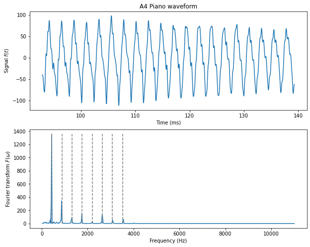
Figure 7.1. Top: The time domain signal of a piano playing the note A4, which has a frequency of 440 Hz. Note that this waveform has some bumpy features and longer modulations that are not straightforward to interpret.
Bottom: The frequency domain representation of the same note. Notice the sharp peaks occurring at regular 440 Hz intervals. The first eight are indicated by the dashed lines.
Compare this to the original representation of the audio signal of the piano in the time domain. Here we clearly see that the signal is oscillating but that each oscillation is characterised by a waveform with some rather unpredictable features that are difficult to interpret. On a fine-grained scale, the signal looks bumpy, and it’s a bit difficult to predict exactly where these bumps will occur. On a coarse-grained level, the oscillations seem to be modulating as the amplitudes of the oscillations change unpredictably. This not only makes the signal more difficult to understand, it also makes it much less efficient to encode digitally. We will see now why.
7.2 The basics of signal compression
Entropy coding
The signal at the top of Figure 7.1 has been encoded digitally. This means that it is represented by a series of numbers, called samples, recorded at even intervals of time (in this case 22050 samples per second). The value of the amplitude of each sample must be recorded with some finite degree of accuracy. In this case, the amplitude is stored as an integer in the range \((-128,128)\). That means the digitisation of the signal has introduced an error of roughly \(1\) part in \(256\) for each sample taken. To reduce this error, you can store each sample in terms of a larger range of numbers. But doing so will require more data storage per sample. The amount of bits of data required to store each sample determines the bitrate of the signal, which is just the total number of bits required to store the signal per second. One important goal of signal processing is to reduce the bitrate of a signal without affecting the quality of the signal.
The simplest way to do this is to notice that signals that don’t change very rapidly require less storage space per sample. Consider the Fourier transform at the bottom of Figure 7.1. Most of the spectrum is almost completely flat. Above 4000 Hz, the Fourier transformed signal stays below a value of \(8\). For all of these frequencies it would be much more efficient to store each sampled frequency using a number in the range \((0,7)\). You could thus store exactly the same signal at a much smaller bitrate.
The process of storing signals by adjusting the bitrate to the flatness of the signal is called entropy coding. Clearly no information is lost in such a coding because you are still storing the same values for each sample. This is called lossless compression because no information is lost in the compression process. However, the amount of compression that is possible depends entirely on the properties of the signal. For the flat Fourier transform at the bottom of Figure 7.1, entropy coding gives an enormous savings of storage since the signal itself is mostly flat. Contrastingly, the original signal is constantly changing between nearly the full range of values \((-128, 128)\). This means that most samples will have to be stored with nearly the full bitrate for each sample. Thus, entropy coding will provide almost no additional savings of storage in this case.
The amount of compression provided by entropy coding can be roughly quantified by a function of the signal called its spectral flatness.2 The less spectrally flat a signal, the less information is required to store the signal, and therefore the more compression you get from entropy coding. One of the main benefits of the Fourier transform is that it is usually much more spiky, and therefore less spectrally flat, than the original signal. This means that, by taking the Fourier transform of a signal, you get bigger compression effects when entropy coding.
Perceptual models for audio signals: the threshold in quiet
To get more significant compression one can eliminate aspects of the signal that don’t affect its overall quality. This is called lossy compression because information is lost in the signal. The secret to lossy compression is to know what aspects of the signal can be thrown away without affecting the signal’s purpose. This, in turn, requires an understanding of the signal and how it’s being used.
As an example, let us consider audio signals. In this case, the signal represents a sound wave that is fed into a speaker to be heard by a human. Any sounds that cannot be heard by the human ear can be removed from the signal without any loss of quality.
The challenge, then, is to determine what sounds cannot be heard by the (typical) human ear. In general, this requires a perceptual model of the human auditory system. In the simplest model, all sounds that are too soft to be heard are removed. To build such a model, all we have to do is measure how loud a particular frequency needs to be before a typical human can just barely detect it. Frequencies outside a certain range, for example those of a dog whistle, cannot be detected no matter how loud they are. But inside this range, there is a threshold that can be measured below which a pure tone of any frequency cannot be heard. This threshold is called the human threshold in quiet. It is measured at a particular frequency with no other sounds present to drown it out. The threshold in quiet is measured in decibels (dB) and is approximated by the following function: \[\begin{equation} \tag{7.2} T(f) = A f^{-4/5} - B e^{-3/5(f - f_0)^2} + C f^4\,, \end{equation}\] where \(A = 3.64\), \(B = 6.5\), \(C = 10^{-3}\), \(f_0 = 3.3\) and the frequency \(f\) is in kHz. This function is shown in Figure 7.2.
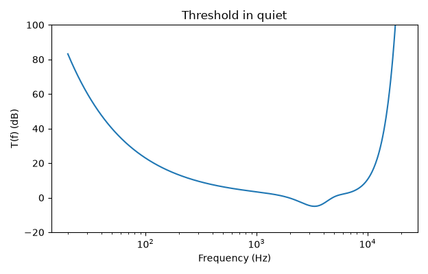
Figure 7.2. The threshold in quiet, Equation (7.2). The formula is from Bosi and Goldberg (2003) (see Sources and Attribution).
To compress a signal, one can simply compare the amplitude of the Fourier transform converted into dB with those of the threshold \(T(f)\) and throw away any that fall below it. This will not lead to any perceptual loss of quality because these signals are imperceptible to the human ear.3 By throwing away the frequencies that can’t be heard, we compress the signal by reducing the number of frequencies to store in memory.
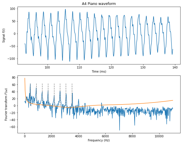
This simple algorithm can be applied to the signal shown in Figure 7.1. Figure 7.3 shows the signal (top) and its Fourier transform (bottom) converted into decibels following the prescription described in Footnote 3. The orange line is the function \(T(f)\) of (7.2) representing the threshold in quiet. Only \(11\%\) of the frequencies in this signal rise above \(T(f)\). For such a simple signal, this results in a significant amount of compression: roughly a factor of \(9\) compression.4
7.3 Filters
The compression algorithm described in the section on the threshold in quiet requires the ability to perform a Fourier transform on some input signal. For many applications, like audio and video streaming, the encoding and decoding must be done in real time. While this is fast enough to do on a modern computer equipped with the right coding libraries — especially after the development of the so-called Fast Fourier Transform (FFT) algorithm — this hasn’t always been the case. In the past, and even for some modern applications such as hearing aids, it is therefore useful to have other methods for isolating the Fourier components of a signal.
What we require is an electronic device that can output a signal whose Fourier transform has effectively been multiplied by a function that drops smoothly to zero in a certain frequency range. A device that achieves this is called a filter because it “filters” out frequencies that lie in a specified range.
There are three different kinds of filters that correspond to the kinds of frequencies the filter cuts out. A filter that removes high frequencies is called a low-pass filter because only frequencies below a certain threshold, \(\omega_0\), are allowed to “pass” through. Conversely, a high-pass filter removes low frequencies and allows frequencies above the threshold, \(\omega_0\), to pass. Finally a band-pass filter only allows frequencies that fall into a certain range \((\omega_0 - \Delta \omega/2, \omega_0 + \Delta \omega/2)\) to pass. In this notation, \(\omega_0\) is in the middle of the frequency “band” and \(\Delta \omega\) is the width of the band.
Mathematically, each of the filters above has the effect of multiplying the Fourier transform of a signal \(F(\omega)\) by some function \(h(\omega)\) so that \(F(\omega) \to h(\omega) F(\omega)\). The function \(h(\omega)\) is itself the Fourier transform as the so-called linear response function of a filter. We can therefore characterise a filter by \(h(\omega)\). This function might have different properties for different kinds of filters but the universal features that distinguish low, high and band pass filters are the following: \[\begin{equation} \tag{7.3} \begin{aligned} h(\omega) &\approx 1 \text{ for } \omega \ll \omega_0 \\ &\approx 0 \text{ for } \omega \gg \omega_0 \end{aligned} \qquad \text{(low-pass)} \end{equation}\] \[\begin{equation} \tag{7.4} \begin{aligned} h(\omega) &\approx 0 \text{ for } \omega \ll \omega_0 \\ &\approx 1 \text{ for } \omega \gg \omega_0 \end{aligned} \qquad \text{(high-pass)} \end{equation}\] \[\begin{equation} \tag{7.5} \begin{aligned} h(\omega) &\approx 1 \text{ for } \omega_0 - \Delta \omega/2 < \omega < \omega_0 + \Delta \omega/2 \\ &\approx 0 \text{ for } \omega \gg \omega_0 \\ &\approx 0 \text{ for } \omega \ll \omega_0 \end{aligned} \qquad \text{(band-pass)} \end{equation}\] We’ll see now that we can build filters with response functions like this using the circuits we’ve studied in this course.
Low-pass filter
First consider the simple RC-circuit shown in Figure 7.4 below. The idea is to apply the signal \(s(t) \equiv v_\text{in}\) as a changing voltage onto the left side of the circuit. We now want to consider the output voltage \(v_\text{out}\) that will be generated across the capacitor. Using the definition of capacitance, we can relate \(v_\text{out}\) to the charge on the capacitor: \(v_\text{out} = Q/C\). Similarly, using Ohm’s law, we can relate the voltage across the resistor to the current \(I = \frac{\mathrm{d}Q}{\mathrm{d}t} = C \frac{\mathrm{d}v_\text{out}}{\mathrm{d}t}\), which is just proportional to the time derivative of the output voltage. \[\begin{equation} \tag{7.6} RC \frac{\mathrm{d}v_\text{out}}{\mathrm{d}t} + v_\text{out} = v_\text{in}\,. \end{equation}\]
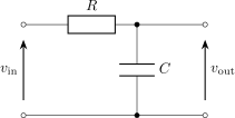
Figure 7.4. An RC circuit set up as a low-pass filter.
The Fourier transform is a very useful tool for solving this differential equation as long as we assume that the signal \(v_\text{in}\) drops to zero outside of some time interval \((t_s, t_f)\). Let us rewrite the input and output signals using the (inverse) Fourier transforms \(\tilde v_\text{in}\) and \(\tilde v_\text{out}\) defined as \[\begin{equation} \tag{7.7} \begin{aligned} v_\text{in}(t) &= \frac 1 {2\pi} \int_{-\infty}^\infty e^{i\omega t} \tilde v_\text{in} \mathrm{d}\omega\,, \\ v_\text{out}(t) &= \frac 1 {2\pi} \int_{-\infty}^\infty e^{i\omega t} \tilde v_\text{out} \mathrm{d}\omega\,. \end{aligned} \end{equation}\] When this is inserted into (7.6) the following algebraic equation is obtained: \[\begin{equation} \tag{7.8} \tilde v_\text{out} = \left(\frac{ 1 }{ 1 + i \tfrac{\omega}{\omega_0} } \right) \tilde v_\text{in}\,, \end{equation}\] where \(\omega_0 = \frac 1 {RC}\) is the cut-off frequency of the filter.
To understand why the circuit in Figure 7.4 is a low-pass filter, we can note that the circuit has the effect of multiplying the Fourier transform of the input signal by the function \[\begin{equation} \tag{7.9} h(\omega) = \frac{ 1 }{ 1 + i \tfrac{\omega}{\omega_0} }\,. \end{equation}\] The amplitude of this function is: \[\begin{equation} \tag{7.10} |h(\omega)| = \frac 1 {\sqrt{1 + \left( \omega/\omega_0\right)^2}}\,. \end{equation}\] This circuit therefore behaves like a low-pass filter because for \(\omega \ll \omega_0\), \(|h(\omega)| \to 1\) and for \(\omega \gg \omega_0\), \(|h(\omega)| \to 0\) as required by (7.3). Note that \(|h|\) does not switch abruptly from \(1\) to \(0\): the transition is spread over a range of frequencies comparable to \(\omega_0\) itself, so this simple circuit is only a rough approximation to an ideal low-pass filter. Sharper cutoffs require more complicated circuits (see the last subsection below).
High-pass filter
We can create a high-pass filter using the RC-circuit shown in Figure 7.5. Kirchhoff’s second law for that circuit gives: \(Q/C + v_\text{out} = v_\text{in}\). Taking time derivatives of this equation and using the fact that \(\frac {\mathrm{d}Q}{\mathrm{d}t} = v_\text{out}/R\) we obtain the following differential equation for \(v_\text{out}\): \[\begin{equation} \tag{7.11} \frac{\mathrm{d}v_\text{out}}{\mathrm{d}t} + \frac{v_\text{out}}{RC} = \frac{\mathrm{d}v_\text{in}}{\mathrm{d}t}\,. \end{equation}\]
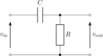
Figure 7.5. An RC circuit set up as a high-pass filter.
Using the (inverse) Fourier transform definition (7.7), this leads to the following Fourier transform of the linear response function \[\begin{equation} \tag{7.12} h(\omega) = \frac {\tilde v_\text{out}}{\tilde v_\text{in}} = \frac { i \omega/\omega_0 }{ 1+ i \omega/\omega_0 }\,, \end{equation}\] which has an amplitude \[\begin{equation} \tag{7.13} |h(\omega)| = \frac { \omega/\omega_0 }{ \sqrt{ 1 + (\omega/\omega_0)^2 } }\,. \end{equation}\] This amplitude goes to zero when \(\omega \ll \omega_0\) and one when \(\omega \gg \omega_0\). The circuit thus behaves like a high-pass filter according to our requirement (7.4).
Band-pass filters
We can construct a band-pass filter using the RLC-circuit of Figure 7.6. In this case, the output voltage is measured across the resistor. Kirchhoff’s second law gives \[\begin{equation} \tag{7.14} L \frac{\mathrm{d}I}{\mathrm{d}t} + \frac Q C + v_\text{out} = v_\text{in}\,. \end{equation}\] Differentiating once and multiplying by \(R/L\) gives the following differential equation for \(v_\text{out}\): \[\begin{equation} \tag{7.15} \frac{\mathrm{d}^2 v_\text{out}}{\mathrm{d}t^2} + \Delta \omega \frac{\mathrm{d}v_\text{out}}{\mathrm{d}t} + \omega_0^2 v_\text{out} = \Delta \omega \frac{ \mathrm{d}v_\text{in} }{\mathrm{d}t}\,, \end{equation}\] where \[\begin{equation*} \omega_0 = \frac 1 {\sqrt{LC}}\,, \qquad \Delta \omega = \frac R L\,. \end{equation*}\] Using the inverse Fourier transforms as before leads to the following response function on Fourier space \[\begin{equation} \tag{7.16} h(\omega) = \frac {i \omega \Delta \omega} { (\omega_0^2 - \omega^2) + i \omega \Delta \omega }\,, \end{equation}\] which has amplitude \[\begin{equation} \tag{7.17} |h(\omega)| = \frac 1 { \sqrt{ \left( \frac{ \omega_0^2 - \omega^2 }{ \omega \Delta \omega } \right)^2 + 1 } }\,. \end{equation}\] Provided we choose \(R\), \(L\), and \(C\) to be such that \(\Delta \omega < \omega_0\), then this amplitude will go to zero when \(\omega \gg \omega_0\) and \(\omega \ll \omega_0\). When \(\omega = \omega_0\), \(|h(\omega)| = 1\). This means that the response function allows frequencies within a band of rough size \(\Delta \omega\) around \(\omega_0\) and stops frequencies outside that band. This is exactly what one would expect for a band-pass filter according to our requirement (7.5).
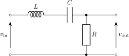
Figure 7.6. An RLC circuit set up as a band-pass filter.
Note that this has the same interpretation as the resonance of the driven RLC circuit, discussed in the section on resonance of the chapter on RL, RLC and AC circuits, and as Equation (15.15) of the OpenStax University Physics Volume 2 online book used in this course. The width \(\Delta\omega = R/L\) is the same width as there, and the quality factor of the circuit is \(\mathsf{Q} = \omega_0/\Delta\omega\). This is because, if we adjust the circuit such that \(\Delta \omega \ll \omega_0\), this frequency response curve will be highly peaked on \(\omega_0\). This means that the circuit is tuned to, or resonating at, the frequency \(\omega_0\).
Signal processing with filters
Using various combinations of low, high and band pass filters, it is possible to isolate and eliminate frequencies in the same way this is done directly with a Fourier transform. Note also that more complicated versions of these circuits can be used to provide cleaner realisations of the functions satisfying (7.3), (7.4) and (7.5). It is even possible to add amplification to the signal, as one might do in a radio receiver. Thus, any compression technique based on a perceptual model of the human auditory system can be implemented using electronic circuits of the kind discussed here. Ultimately, this is because the human auditory system itself is effectively a system of mechanical and electrical filters that performs its own processing on the sounds waves entering the ear. The goal of compression algorithms is to mimic this processing and eliminate any information that is unnecessary.
Early compression algorithms, like MPEG 1 and 2,5 run the signal through an array of \(32\) band-pass filters centred on evenly spaced frequency intervals. This array of filters is called a filter-bank. These different bands are supposed to mimic the different absorption bands found in the inner ear. One can then analyse the signal in each of these bands and determine which ones are either below the threshold in quiet or are drowned out by louder sounds in neighbouring bands.6 The bands that are found to be too soft to be heard can then either be eliminated or stored at a much lower band-width than the original signal. During playback, the 32 bands are recombined to produce a sound that is imperceptibly different from the original but that is much more spectrally flat and, therefore, takes much less memory to store. More modern formats like MP4, use Fast Fourier Transform algorithms to analyse and manipulate the signal directly in Fourier space. This requires faster computing power that is not always available for smaller devices like hearing aids. The underlying mathematical principles, however, are the same.
Note that this condition follows trivially from taking the complex conjugate of the definition, (6.7), of the Fourier transform.↩︎
Formally, the spectral flatness is defined as the ratio of the geometric and arithmetic means \(= \frac{ \left( \prod x_n \right)^{1/N} }{ \frac 1 N \sum x_n }\), where \(x_n\) is the \(n^\text{th}\) sample of the signal and \(N\) is the total number of samples. It has a maximum at \(1\), which is approached for white noise, and a minimum at zero.↩︎
In practice, converting a Fourier transform into decibels, dB, is done by taking \(\text{dB} = 20 \log_{10} A\), where \(A\) is the amplitude of the Fourier transform of a pure sine wave with amplitude equal to the smallest signal that can be recorded at the given bitrate (eg, the amplitude of this smallest sine wave is \(1\) for the signal of Figure 7.1). This somewhat arbitrary definition is suitable for most purposes as long as the gain of the amplified audio output produces a sound with a comfortable listening volume.↩︎
Note that the signal at the frequencies that do remain is large and will typically require more memory than each sample of the original signal so that the exact compression factor is tricky to calculate.↩︎
For example, files with the ‘MP3’ file extensions↩︎
This is a phenomenon called masking.↩︎