Chapter 6
Fourier Series
6.1 Fourier series
Consider a periodic function \(s(t)\) that repeats outside the interval \(t\in[-L,L]\) and satisfies:
\(\displaystyle\int_{-L}^{L} |s(t)|\,dt < \infty\),
\(s(t)\) has a finite number of discontinuities,
\(s(t)\) has a finite number of extrema.
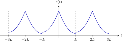
Note: \(s(t)\) could also just be defined only on \([-L,L]\).
Then it is possible to write \(s(t)\) as an infinite sum of sine and cosine functions: \[\begin{equation} \tag{6.1} \keyeq{\displaystyle s(t) = \frac{a_0}{2} + \sum_{n=1}^{\infty}\left[a_n\cos\!\left(\frac{\pi n t}{L}\right) + b_n\sin\!\left(\frac{\pi n t}{L}\right)\right]} \end{equation}\]
Idea: the coefficients \((a_n,b_n)\) are like the “components” of an infinite-dimensional “vector”, where the orthonormal “basis” elements are sines and cosines. For example, a vector in three dimensions is \(\vec v = v_x\,\hat\imath + v_y\,\hat\jmath + v_z\,\hat k\): \[(v_x,v_y,v_z)\;\to\;(a_n,b_n), \qquad (\hat\imath,\hat\jmath,\hat k)\;\to\;(\sin,\cos).\]
Orthogonality
Here the inner product is now an integral over \([-L,L]\). For vectors, \(\langle\vec v,\vec u\rangle = \sum_i v_iu_i\); for functions \[\langle s(t), r(t)\rangle = \frac{1}{L}\int_{-L}^{L} s(t)\,r(t)\,dt\,.\] For the unit vectors, \(\hat\imath\cdot\hat\imath = \hat\jmath\cdot\hat\jmath = \hat k\cdot\hat k = 1\) and \(\hat\imath\cdot\hat\jmath = \hat\jmath\cdot\hat k = \hat\imath\cdot\hat k = 0\). The sines and cosines satisfy the same relations, for integers \(m,n\ge 1\): \[\begin{equation} \tag{6.2} \keyeq{\displaystyle \frac1L\int_{-L}^{L}dt\,\sin\!\left(\frac{m\pi t}{L}\right)\sin\!\left(\frac{n\pi t}{L}\right) = \delta_{mn}} \end{equation}\] \[\begin{equation} \tag{6.3} \keyeq{\displaystyle \frac1L\int_{-L}^{L}dt\,\cos\!\left(\frac{m\pi t}{L}\right)\cos\!\left(\frac{n\pi t}{L}\right) = \delta_{mn}} \end{equation}\] \[\begin{equation} \tag{6.4} \keyeq{\displaystyle \frac1L\int_{-L}^{L}dt\,\sin\!\left(\frac{m\pi t}{L}\right)\cos\!\left(\frac{n\pi t}{L}\right) = 0} \end{equation}\] Check. Use \(\sin A\sin B = \tfrac12[\cos(A-B)-\cos(A+B)]\). For \(m\neq n\) both cosines integrate to zero over a whole number of periods; for \(m=n\) the first term is \(1\) and the second integrates to zero, so the integral is \(\frac{1}{L}\cdot\frac12\cdot 2L = 1\). The cosine–cosine case is identical with \(\cos A\cos B = \tfrac12[\cos(A-B)+\cos(A+B)]\), and the sine–cosine integrand is odd, so it integrates to zero over the symmetric interval.
The coefficients
Multiply (6.1) by \(\cos(m\pi t/L)\) and integrate. For \(m\neq 0\), using (6.3) and (6.4): \[\frac1L\int_{-L}^{L}dt\,s(t)\cos\!\left(\frac{m\pi t}{L}\right) = \frac1L\int_{-L}^{L}dt\sum_{n=1}^{\infty}\left[a_n\cos\!\left(\frac{n\pi t}{L}\right)+b_n\sin\!\left(\frac{n\pi t}{L}\right)\right]\cos\!\left(\frac{m\pi t}{L}\right) = \sum_{n=1}^{\infty}\left(a_n\delta_{mn}+0\right) = a_m\,.\] For \(m=0\): \[\frac1L\int_{-L}^{L}dt\,s(t) = \frac1L\int_{-L}^{L}\frac{a_0}{2}\,dt = \frac{a_0}{2}\cdot\frac{2L}{L} = a_0\,.\] Similarly, using (6.2) and (6.4), \[\frac1L\int_{-L}^{L}dt\,s(t)\sin\!\left(\frac{m\pi t}{L}\right) = 0 + \sum_{n=1}^{\infty}\left(0+b_n\delta_{mn}\right) = b_m\,.\] Collecting these results: \[\begin{equation} \tag{6.5} \keyeq{\displaystyle a_n = \frac1L\int_{-L}^{L}dt\,s(t)\cos\!\left(\frac{n\pi t}{L}\right),\quad n\ge 0} \end{equation}\] \[\begin{equation} \tag{6.6} \keyeq{\displaystyle b_n = \frac1L\int_{-L}^{L}dt\,s(t)\sin\!\left(\frac{n\pi t}{L}\right),\quad n\ge 1} \end{equation}\]
6.2 Example: the step function
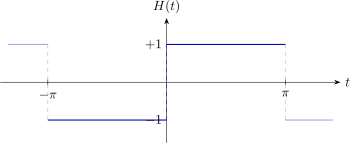
Take \(L=\pi\) and \(s(t)=H(t)\), where \[H(t) = \begin{cases} -1, & -\pi < t < 0,\\ +1, & 0 < t < \pi. \end{cases}\]
Since \(H\) is odd and \(\cos(nt)\) is even, the integrand of \(a_n\) is odd and \[a_n = \frac1\pi\int_{-\pi}^{\pi}dt\,H(t)\cos(nt) = 0\,.\] For \(b_n\) the integrand is even (odd \(\times\) odd), so we can double the integral over \([0,\pi]\): \[b_n = \frac1\pi\int_{-\pi}^{\pi}dt\,H(t)\sin(nt) = \frac{2}{\pi}\int_0^{\pi}dt\,\sin(nt) = -\frac{2}{\pi}\,\frac{\cos(nt)}{n}\bigg|_0^{\pi} = \frac{2}{n\pi}\left(1-(-1)^n\right),\] using \(\cos(n\pi)=+1\) for even \(n\) and \(-1\) for odd \(n\), and \(\cos 0 = 1\). Hence \[b_n = \begin{cases} \dfrac{4}{n\pi}, & n \text{ odd},\\[2mm] 0, & n\text{ even}, \end{cases} \qquad\text{so}\qquad H(t) = \frac4\pi\left[\sin t + \frac{\sin 3t}{3} + \frac{\sin 5t}{5} + \cdots\right].\]
6.3 From Fourier series to the Fourier transform
The Fourier series (6.1) describes a function that repeats with period \(2L\). A signal that does not repeat, such as a single pulse, can be thought of as the limit \(L\to\infty\) of a periodic one. Let us see what happens to the series in this limit.
Complex form
Write \(\omega_n = n\pi/L\) for the frequency of the \(n\)th term. Then (6.1), (6.5) and (6.6) read \[s(t) = \frac{a_0}{2} + \sum_{n=1}^{\infty}\left[a_n\cos(\omega_n t) + b_n\sin(\omega_n t)\right], \qquad \begin{aligned} a_n &= \frac1L\int_{-L}^{L}dt'\,s(t')\cos(\omega_n t'),\\ b_n &= \frac1L\int_{-L}^{L}dt'\,s(t')\sin(\omega_n t'). \end{aligned}\] The neighbouring frequencies are separated by \(\Delta\omega = \omega_{n+1}-\omega_n = \pi/L\). Combine the two coefficients into one complex number, \[F_n \equiv a_n - i\,b_n = \frac1L\int_{-L}^{L}dt'\,s(t')\left[\cos(\omega_n t') - i\sin(\omega_n t')\right] = \frac1L\int_{-L}^{L}dt'\,s(t')\,e^{-i\omega_n t'},\] where we used Euler’s formula \(e^{i\theta}=\cos\theta + i\sin\theta\). Since \((a_n - i b_n)\,e^{i\omega_n t} = a_n\cos(\omega_n t) + b_n\sin(\omega_n t) + i\left[a_n\sin(\omega_n t) - b_n\cos(\omega_n t)\right]\), each term of the series is the real part of \(F_n e^{i\omega_n t}\): \[s(t) = \frac{a_0}{2} + \sum_{n=1}^{\infty}\mathrm{Re}\!\left[F_n\,e^{i\omega_n t}\right].\]
The limit \(L\to\infty\)
As \(L\) grows, the coefficients \(F_n\) shrink like \(1/L\), so we define the rescaled quantity \(F(\omega_n) \equiv L\,F_n\), which stays finite. Using \(1/L = \Delta\omega/\pi\) the series becomes \[s(t) = \frac{a_0}{2} + \frac1\pi\sum_{n=1}^{\infty}\mathrm{Re}\!\left[F(\omega_n)\,e^{i\omega_n t}\right]\Delta\omega\,, \qquad F(\omega_n) = \int_{-L}^{L}dt'\,s(t')\,e^{-i\omega_n t'}.\] When \(L\to\infty\):
the spacing \(\Delta\omega=\pi/L\to 0\), so the allowed frequencies \(\omega_n = n\Delta\omega\) fill out a continuous variable \(\omega\) and the sum over \(n\) becomes an integral over \(\omega\in(0,\infty)\);
\(a_0/2 = \frac{1}{2L}\int s\,dt \to 0\), because \(\int|s|\,dt\) is finite.
We therefore obtain the Fourier transform of \(s(t)\), \[\begin{equation} \tag{6.7} \keyeq{\displaystyle F(\omega) = \int_{-\infty}^{\infty}dt\,s(t)\,e^{-i\omega t}} \end{equation}\] and the representation of the signal \[s(t) = \frac1\pi\,\mathrm{Re}\int_0^\infty d\omega\,F(\omega)\,e^{i\omega t}.\]
The inverse transform
Since \(s(t)\) is real, complex conjugating (6.7) gives \(F(\omega)^\star = F(-\omega)\). The complex conjugate of the integrand \(F(\omega)e^{i\omega t}\) is therefore \(F(-\omega)e^{-i\omega t}\), and \(\mathrm{Re}\,z=\tfrac12(z+z^\star)\) gives \[\mathrm{Re}\int_0^\infty d\omega\,F(\omega)e^{i\omega t} = \frac12\int_0^\infty d\omega\,F(\omega)e^{i\omega t} + \frac12\int_0^\infty d\omega\,F(-\omega)e^{-i\omega t} = \frac12\int_{-\infty}^{\infty}d\omega\,F(\omega)e^{i\omega t},\] where the second term was rewritten by substituting \(\omega\to-\omega\). Hence \[\begin{equation} \tag{6.8} \keyeq{\displaystyle s(t) = \frac{1}{2\pi}\int_{-\infty}^{\infty}d\omega\,F(\omega)\,e^{i\omega t}} \end{equation}\] Compare this with the Fourier series: the discrete frequencies \(\omega_n\) and coefficients \((a_n,b_n)\) have been replaced by a continuous frequency \(\omega\) and the complex function \(F(\omega)\), whose real part plays the role of \(a_n\) and minus its imaginary part that of \(b_n\) (up to the overall factor \(L\)). The signal conditions are the same as for the series, with \(\int_{-\infty}^{\infty}|s(t)|\,dt<\infty\).
Problems
Problems are taken from the sources listed under Sources and Attribution. Numbers refer to the end-of-chapter problems; figures have been redrawn.
Fourier problem set
These problems are from the course (not from the sources above).
1
(a) Plot the waveform of the periodic function defined as \[f(t) = -\frac{2t}{\pi}\quad\text{if}\quad -\pi\le t\le\pi, \qquad f(t) = f(t+2\pi)\ \text{ for all } t\,.\]
(b) Compute the Fourier series of this function for all \(n\).
2
(a) Using the provided python code (the interactive tool below), plot the ‘sawtooth’ waveform as a function of time for a value of \(w\) not equal to zero, one or \(1/2\). Try to pick a value that will highlight interesting features of the Fourier series and explain why you made your choice. What is special about the values \(w=0\), \(w=1/2\) and \(w=1\)?
(b) For the value of \(w\) chosen above, plot the Fourier coefficients for up to \(N=15\).
(c) Choose \(3\) values of \(N\) (different from \(15\)) for which to plot the \(N^{\text{th}}\) order Fourier approximation that illustrate different characteristics of the approximation. Explain what is happening as \(N\) gets large and why you chose the values you did.
3
Use the interactive tool above (choose the waveform from problem 1) to check your answer to problem 1. Make a plot to compare the analytic solution obtained to the numerical computation (by plotting the difference, plotting them side-by-side, or some other way).