Chapter 1
Electric Fields & Capacitance
1.1 Electric field
The electric field \(\vb E(\vb x,t)\) maps a point \(\vb x\) and a time \(t\) to a vector \(\vb E\).
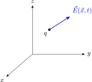
Physically: \(\vb E\) tells us how a test charge will move when placed at \(\vb x\). The force on a test particle of charge \(q\) is \[\begin{equation} \tag{1.1} \keyeq{\vb F = q\,\vb E} \qquad\Longleftrightarrow\qquad \vb E = \frac{\vb F}{q}. \end{equation}\]
Electric charge
Electric charge plays two roles:
it is the propensity for producing an electric field;
it determines the force, \(\vb F\) in response to an applied electric field. From (1.1), \(q = |\vb F|/|\vb E|\).
Charges, at rest or in motion, are the sources of all electromagnetic fields.
1.2 Coulomb’s law
Coulomb’s law gives the electric force \(\vb F_E\) that static point charges (i.e. in vacuum, at rest) exert on other charges.
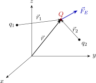
\[\begin{equation} \tag{1.2} \keyeq{\displaystyle \vb F_E(\vb r) = \frac{Q}{4\pi\varepsilon_0}\sum_i \frac{q_i}{r_i^2}\,\uv r_i} \end{equation}\]
where
\(Q\) is the charge of the particle experiencing \(\vb F_E\);
\(\vb r_i\) is the separation vector from charge \(q_i\) to \(Q\), with length \(r_i = |\vb r_i|\) and unit vector \(\displaystyle \uv r_i = \frac{\vb r_i}{|\vb r_i|}\);
\(\varepsilon_0\) is the permittivity of free space, \(\varepsilon_0 = 8.854\times 10^{-12}\,\mathrm{F/m}\).
Combining (1.1) and (1.2) gives the electric field produced by \(N\) charged particles: \[\keyeq{\displaystyle \vb E(\vb r) = \frac{\vb F_E}{Q} = \frac{1}{4\pi\varepsilon_0}\sum_{i=1}^{N}\frac{q_i}{r_i^2}\,\uv r_i}\]
Example: two equal charges
Two charges \(q\) sit on the \(x\)-axis at \(x=\pm L\). Find the field at point \(P\), a height \(D\) above their midpoint.
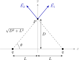
By superposition, \(\vb E(P) = \vb E_1 + \vb E_2 = (E_x^1 + E_x^2)\,\uv\imath + (E_y^1 + E_y^2)\,\uv\jmath\). By symmetry \(E_x^2 = -E_x^1\) and \(E_y^2 = E_y^1\), so \[\vb E(P) = 2E_y^1\,\uv\jmath .\] With \(\sin\theta = D/\sqrt{D^2+L^2}\) and \(r_1^2 = D^2+L^2\), \[E_y^1 = \frac{q}{4\pi\varepsilon_0}\,\frac{\sin\theta}{r_1^2} = \frac{q}{4\pi\varepsilon_0}\,\frac{D}{(D^2+L^2)^{3/2}} ,\] and therefore \[\keyeq{\displaystyle \vb E(P) = \frac{q}{2\pi\varepsilon_0}\,\frac{D}{(D^2+L^2)^{3/2}}\;\uv\jmath}\]
1.3 Voltage
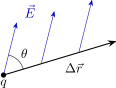
\(|\Delta \vb r| = d\)
Work done by the electric force on \(q\) as it moves through \(\Delta\vb r\) in a uniform field: \[W_E = \vb F_E\cdot\Delta\vb r = q\,E\,d\cos\theta .\]
The electric potential difference, a.k.a. “voltage”, is the (negative of the) work done per unit charge: \[\begin{equation} \tag{1.3} \keyeq{\displaystyle \Delta V = -\frac{W_E}{q} = -E\,d\cos\theta} \end{equation}\]
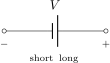
A battery is a device that maintains a potential difference \(V\) between two conducting terminals. Its circuit symbol has two parallel lines of unequal length: the longer line is the positive terminal (higher potential) and the shorter line is the negative terminal (lower potential), so \(V = V_+ - V_-\). We’ll use this symbol for any constant voltage source.
1.4 Capacitors
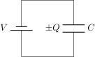
A capacitor is made of two conducting plates across which a voltage \(V\) can be applied. One plate acquires charge \(+Q\), the other \(-Q\).
Capacitance: \(\keyeq{\displaystyle C = \frac{Q}{V} = \frac{\text{charge on plate}}{\text{voltage}}}\)
Units: farad, \(\mathrm{F} = \mathrm{C/V}\).
Parallel-plate capacitor
For a parallel-plate capacitor with plate area \(A\) and separation \(d\), the field between the plates is uniform: \[E = \frac{Q}{\varepsilon_0 A}.\] Using (1.3) (magnitude, with \(\theta=0\)), \(V = Ed\), so \[C_{\parallel} = \frac{Q}{V} = \frac{Q}{Ed} = \frac{Q}{\dfrac{Q}{\varepsilon_0 A}\,d} \quad\Longrightarrow\quad \keyeq{\displaystyle C_{\parallel} = \frac{\varepsilon_0 A}{d}}\] Note that \(Q\) cancels: capacitance depends only on geometry (a general result).
Capacitors in series
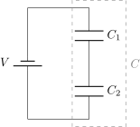
Let \(C\) be the effective capacitance of the combination.
Conservation of energy (Kirchhoff’s voltage law): \(V_1 + V_2 = V\).
Conservation of charge: the inner plates carry equal and opposite charge, \(Q_1^+ = -Q_2^-\), so both capacitors hold the same \(Q\).
\[C_1 = \frac{Q}{V_1}, \qquad C_2 = \frac{Q}{V_2} \qquad\Longrightarrow\qquad C = \frac{Q}{V} = \frac{Q}{\dfrac{Q}{C_1}+\dfrac{Q}{C_2}} = \frac{1}{\dfrac{1}{C_1}+\dfrac{1}{C_2}}\] \[\keyeq{\displaystyle \frac{1}{C} = \frac{1}{C_1} + \frac{1}{C_2}}\]
Capacitors in parallel
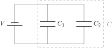
Here the charges add and the voltages are equal: \[Q = Q_1 + Q_2, \qquad V_1 = V_2 = V.\] So \[C = \frac{Q}{V} = \frac{Q_1+Q_2}{V} = C_1 + C_2 ,\] \[\keyeq{C = C_1 + C_2}\]
Example
Find the effective capacitance of the circuit below.
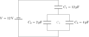
\(C_2\) and \(C_3\) are in parallel, so they combine to \(C_4 = C_2 + C_3 = 6\,\mathrm{\mu F}\). \(C_4\) is then in series with \(C_1\): \[\frac{1}{C} = \frac{1}{C_1} + \frac{1}{C_4} \;\Longrightarrow\; C = \frac{C_1 C_4}{C_1 + C_4} = \frac{12\cdot 6}{12+6}\,\mathrm{\mu F} \qquad\Longrightarrow\qquad \keyeq{C = 4\,\mathrm{\mu F}}\]
Problems
Problems are taken from the sources listed under Sources and Attribution. Numbers refer to the end-of-chapter problems; figures have been redrawn.
OpenStax University Physics Vol. 2, Chapter 5: Electric Charges and Fields
5.53
Point charges \(q_1 = 50\,\mathrm{\mu C}\) and \(q_2 = -25\,\mathrm{\mu C}\) are placed \(1.0\,\mathrm{m}\) apart. What is the force on a third charge \(q_3 = 20\,\mathrm{\mu C}\) placed midway between \(q_1\) and \(q_2\)?
5.63
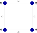
What is the force on the charge \(q\) at the lower-right-hand corner of the square shown here?
5.95
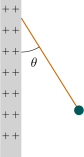
Shown is a small sphere of mass \(0.25\,\mathrm{g}\) that carries a charge of \(9.0\times 10^{-10}\,\mathrm{C}\). The sphere is attached to one end of a very thin silk string \(5.0\,\mathrm{cm}\) long. The other end of the string is attached to a large vertical conducting plate that has a charge density of \(30\times 10^{-6}\,\mathrm{C/m^2}\). What is the angle that the string makes with the vertical?
OpenStax University Physics Vol. 2, Chapter 8: Capacitance
8.27
A set of parallel plates has a capacitance of \(5.0\,\mathrm{\mu F}\). How much charge must be added to the plates to increase the potential difference between them by \(100\,\mathrm{V}\)?
8.33
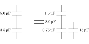
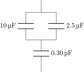
Find the total capacitance of this combination of series and parallel capacitors.
8.37
Find the net capacitance of the combination of series and parallel capacitors shown.